40 data labels on excel chart

How to create Custom Data Labels in Excel Charts - Efficiency 365 Create the chart as usual. Add default data labels. Click on each unwanted label (using slow double click) and delete it. Select each item where you want the custom label one at a time. Press F2 to move focus to the Formula editing box. Type the equal to sign. Now click on the cell which contains the appropriate label. 1/ Select A1:B7 > Inser your Histo. chart. 2/ Right-click i.e. on the 1st histo. bar (A) > Add Data Labels (numbers are displayed a the top of the bars) 3/ Click one of the numbers that just displayed (the Format Data Labels pane opens on the right) > Check option "Value From Cells" > Select range C2:C7 > OK > Uncheck option "Value".

Excel Chart Data Labels - Microsoft Community Right-click a data point on your chart, from the context menu choose Format Data Labels ..., choose Label Options > Label Contains Value from Cells > Select Range. In the Data Label Range dialog box, verify that the range includes all 26 cells. When I paste your data into a worksheet, the XY Scatter data is in A2:B27, and the data labels are in ...

Data labels on excel chart

Customize the vertical axis labels - Microsoft Excel 365 See more about creating a tally chart in Excel. Note: See also how to conditionally highlight axis labels. Add a new data series to the chart. The main purpose of the new data series is to substitute the axis labels - the new data series labels will be displayed instead of the axis labels. How to change Axis labels in Excel Chart - A Complete Guide Right-click the horizontal axis (X) in the chart you want to change. In the context menu that appears, click on Select Data…. A Select Data Source dialog opens. In the area under the Horizontal (Category) Axis Labels box, click the Edit command button. Enter the labels you want to use in the Axis label range box, separated by commas. Custom Chart Data Labels In Excel With Formulas - How To Excel At Excel Follow the steps below to create the custom data labels. Select the chart label you want to change. In the formula-bar hit = (equals), select the cell reference containing your chart label's data. In this case, the first label is in cell E2. Finally, repeat for all your chart laebls.

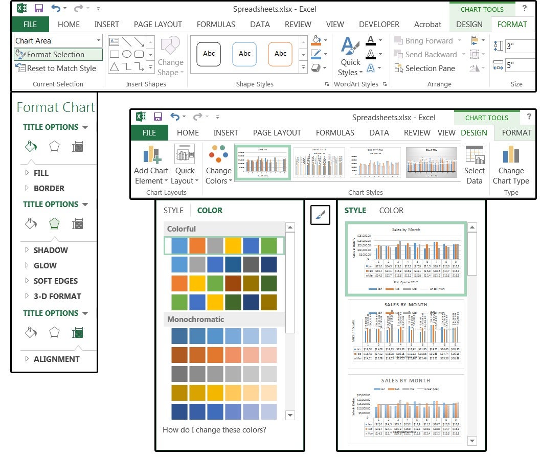
Data labels on excel chart. Change the format of data labels in a chart To get there, after adding your data labels, select the data label to format, and then click Chart Elements > Data Labels > More Options. To go to the appropriate area, click one of the four icons ( Fill & Line, Effects, Size & Properties ( Layout & Properties in Outlook or Word), or Label Options) shown here. How to add total labels to stacked column chart in Excel? - ExtendOffice 1. Create the stacked column chart. Select the source data, and click Insert > Insert Column or Bar Chart > Stacked Column. 2. Select the stacked column chart, and click Kutools > Charts > Chart Tools > Add Sum Labels to Chart. Then all total labels are added to every data point in the stacked column chart immediately. Excel Charts - Aesthetic Data Labels - tutorialspoint.com Data Label Positions To place the data labels in the chart, follow the steps given below. Step 1 − Click the chart and then click chart elements. Step 2 − Select Data Labels. Click to see the options available for placing the data labels. Step 3 − Click Center to place the data labels at the center of the bubbles. Format a Single Data Label How to add data labels from different column in an Excel chart? Right click the data series in the chart, and select Add Data Labels > Add Data Labels from the context menu to add data labels. 2. Click any data label to select all data labels, and then click the specified data label to select it only in the chart. 3.

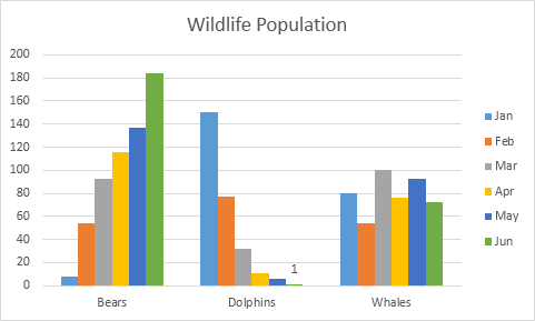
How to add or move data labels in Excel chart? - ExtendOffice In Excel 2013 or 2016. 1. Click the chart to show the Chart Elements button . 2. Then click the Chart Elements, and check Data Labels, then you can click the arrow to choose an option about the data labels in the sub menu. See screenshot: In Excel 2010 or 2007. 1. click on the chart to show the Layout tab in the Chart Tools group. See ... How to☝️Create a Pie of Pie Chart in Excel - SpreadsheetDaddy Data Labels is a feature in Excel that allows you to add labels to data points in your chart. You can use data labels to show the value of each data point as well as the percentage of the total each data point represents. Let's take a look at how to add data points to your chart. Right-click on the chart. Select the Add Data Labels option. How to Use Cell Values for Excel Chart Labels - How-To Geek Select the chart, choose the "Chart Elements" option, click the "Data Labels" arrow, and then "More Options." Uncheck the "Value" box and check the "Value From Cells" box. Select cells C2:C6 to use for the data label range and then click the "OK" button. The values from these cells are now used for the chart data labels. Data Labels in Excel Pivot Chart (Detailed Analysis) 7 Suitable Examples with Data Labels in Excel Pivot Chart Considering All Factors 1. Adding Data Labels in Pivot Chart 2. Set Cell Values as Data Labels 3. Showing Percentages as Data Labels 4. Changing Appearance of Pivot Chart Labels 5. Changing Background of Data Labels 6. Dynamic Pivot Chart Data Labels with Slicers 7.

How to Select Data for Graphs in Excel - Sheetaki Select the blank graph and navigate to the Chart Design tab. Click on the Select Data option. In the Select Data Source dialog box, select the Chart data range text box and type in your range. You may also use your cursor to select the range much faster. Click on the OK button to apply the new data source to your graph. How to Add Two Data Labels in Excel Chart (with Easy Steps) Select the data labels. Then right-click your mouse to bring the menu. Format Data Labels side-bar will appear. You will see many options available there. Check Category Name. Your chart will look like this. Now you can see the category and value in data labels. Read More: How to Format Data Labels in Excel (with Easy Steps) Things to Remember How to hide zero data labels in chart in Excel? - ExtendOffice If you want to hide zero data labels in chart, please do as follow: 1. Right click at one of the data labels, and select Format Data Labels from the context menu. See screenshot: 2. In the Format Data Labels dialog, Click Number in left pane, then select Custom from the Category list box, and type #"" into the Format Code text box, and click Add button to add it to Type list box. How to I rotate data labels on a column chart so that they are ... To change the text direction, first of all, please double click on the data label and make sure the data are selected (with a box surrounded like following image). Then on your right panel, the Format Data Labels panel should be opened. Go to Text Options > Text Box > Text direction > Rotate

Pie Chart - PK: An Excel Expert

Move data labels - support.microsoft.com Click any data label once to select all of them, or double-click a specific data label you want to move. Right-click the selection > Chart Elements > Data Labels arrow, and select the placement option you want. Different options are available for different chart types.

Excel charts: Mastering pie charts, bar charts and more | PCWorld

Edit titles or data labels in a chart - support.microsoft.com On a chart, click one time or two times on the data label that you want to link to a corresponding worksheet cell. The first click selects the data labels for the whole data series, and the second click selects the individual data label. Right-click the data label, and then click Format Data Label or Format Data Labels.

E-xcel Tuts: Add Data Labels to Excel Charts

Add or remove data labels in a chart - support.microsoft.com Click the data series or chart. To label one data point, after clicking the series, click that data point. In the upper right corner, next to the chart, click Add Chart Element > Data Labels. To change the location, click the arrow, and choose an option. If you want to show your data label inside a text bubble shape, click Data Callout.

How-to Use Data Labels from a Range in an Excel Chart - Excel Dashboard Templates

Chart.ApplyDataLabels method (Excel) | Microsoft Docs The type of data label to apply. True to show the legend key next to the point. The default value is False. True if the object automatically generates appropriate text based on content. For the Chart and Series objects, True if the series has leader lines. Pass a Boolean value to enable or disable the series name for the data label.

Excel Solution - How to Create Custom Data Label in Chart.avi - YouTube

Add or remove data labels in a chart This displays the Chart Tools, adding the Design, and Format tabs. On the Design tab, in the Chart Layouts group, click Add Chart Element, choose Data Labels, and then click None. Click a data label one time to select all data labels in a data series or two times to select just one data label that you want to delete, and then press DELETE.

Nested donut chart (also known as Multi-level doughnut chart, Multi-series doughnut chart ...

Data labels on small states using Maps - Microsoft Community Data labels on small states using Maps. Hello, I need some assistance using the Filled Maps chart type in Excel (note: this is NOT Power Maps). I have some data (see attachment below) that I've plotted on a map of the USA. Because the data only applied to 7 states I changed the "map area" (under Format Data Series-->Series Options) to show ...

Charting in Excel - Adding Data Labels - YouTube

how to add data labels into Excel graphs - storytelling with data There are a few different techniques we could use to create labels that look like this. Option 1: The "brute force" technique. The data labels for the two lines are not, technically, "data labels" at all. A text box was added to this graph, and then the numbers and category labels were simply typed in manually.

Custom Data Labels with Colors and Symbols in Excel Charts – [How To] - KING OF EXCEL

Custom Chart Data Labels In Excel With Formulas - How To Excel At Excel Follow the steps below to create the custom data labels. Select the chart label you want to change. In the formula-bar hit = (equals), select the cell reference containing your chart label's data. In this case, the first label is in cell E2. Finally, repeat for all your chart laebls.

Plot Area in Excel and Google Spreadsheets Charts

How to change Axis labels in Excel Chart - A Complete Guide Right-click the horizontal axis (X) in the chart you want to change. In the context menu that appears, click on Select Data…. A Select Data Source dialog opens. In the area under the Horizontal (Category) Axis Labels box, click the Edit command button. Enter the labels you want to use in the Axis label range box, separated by commas.