43 custom data labels excel 2010 scatter plot
Create a chart from start to finish - support.microsoft.com You can create a chart for your data in Excel for the web. Depending on the data you have, you can create a column, line, pie, bar, area, scatter, or radar chart. Click anywhere in the data for which you want to create a chart. To plot specific data into a chart, you can also select the data. How to Create a Stem-and-Leaf Plot in Excel - Automate Excel Step #10: Add data labels. As you inch toward the finish line, let’s add the leaves to the chart. To do that, right-click on any dot representing Series “Series 1” and choose “Add Data Labels.” Step #11: Customize data labels. Once there, get rid of the default labels and add the values from column Leaf (Column D) instead.
Custom Data Labels with Colors and Symbols in Excel Charts - [How To] Step 4: Select the data in column C and hit Ctrl+1 to invoke format cell dialogue box. From left click custom and have your cursor in the type field and follow these steps: Press and Hold ALT key on the keyboard and on the Numpad hit 3 and 0 keys. Let go the ALT key and you will see that upward arrow is inserted.
:max_bytes(150000):strip_icc()/ScatterStyle-Edit-ec1ee3fbd48047e5842b14011ac90f66.jpg)
Custom data labels excel 2010 scatter plot
Add data label when hovering mouse over data points on a XY scatter plot. When I plot a XY scatter plot, and click the chart then hover the mouse pointer over a data point to have excel display Name (X,Y) such as A(1,2). In my case, I can't use any add-in application. The chart is embedded in the worksheet. I am using Excel 2010. Appreciate your help! Thanks, Excel Dashboard Course - My Online Training Hub Power Query gets data from almost any source (a database, the web, Excel, Sharepoint, Salesforce, OData etc), and loads it into Excel or Power Pivot for analysis, report preparation or export. Power Pivot can import millions of rows of data, create relationships between different data sources, and build interactive reports. Notes How to Perform Exploratory Data Analysis with Seaborn Feb 19, 2019 · It is used to understand data, get some context regarding it, understand the variables and the relationships between them, and formulate hypotheses that could be useful when building predictive models. All data analysis must be guided by some key questions or objectives. Before starting any data analysis tasks, you should have a clear goal in mind.
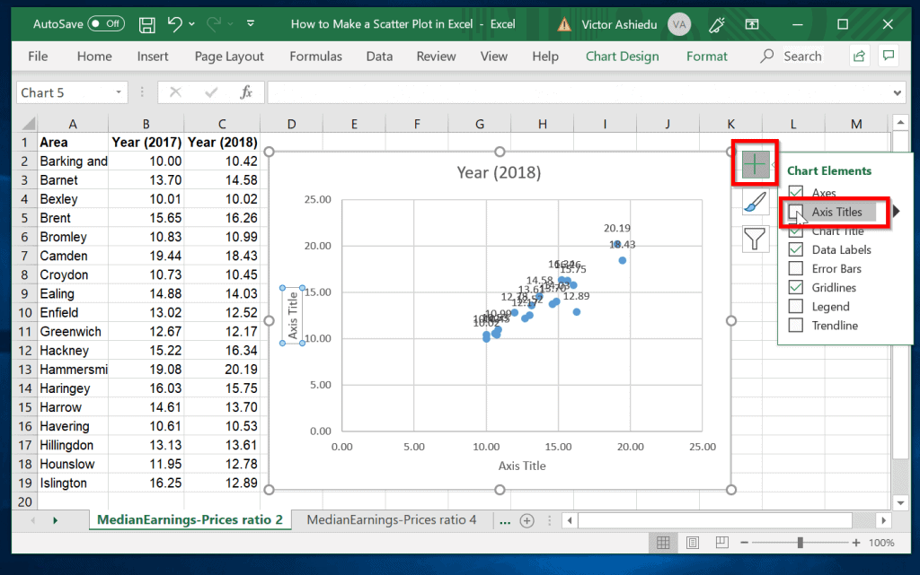
Custom data labels excel 2010 scatter plot. Use text as horizontal labels in Excel scatter plot Edit each data label individually, type a = character and click the cell that has the corresponding text. This process can be automated with the free XY Chart Labeler add-in. Excel 2013 and newer has the option to include "Value from cells" in the data label dialog. Format the data labels to your preferences and hide the original x axis labels. How to use a macro to add labels to data points in an xy scatter chart ... Click Chart on the Insert menu. In the Chart Wizard - Step 1 of 4 - Chart Type dialog box, click the Standard Types tab. Under Chart type, click XY (Scatter), and then click Next. In the Chart Wizard - Step 2 of 4 - Chart Source Data dialog box, click the Data Range tab. Under Series in, click Columns, and then click Next. How can I add data labels from a third column to a scatterplot? Under Labels, click Data Labels, and then in the upper part of the list, click the data label type that you want. Under Labels, click Data Labels, and then in the lower part of the list, click where you want the data label to appear. Depending on the chart type, some options may not be available. Change the format of data labels in a chart To get there, after adding your data labels, select the data label to format, and then click Chart Elements > Data Labels > More Options. To go to the appropriate area, click one of the four icons ( Fill & Line, Effects, Size & Properties ( Layout & Properties in Outlook or Word), or Label Options) shown here.
Macro to add data labels to scatter plot | MrExcel Message Board It's an Excel macro, not something that requires installing. Downloading, yes, but you can put the macro anywhere. In any case, here's the code: Sub AddXYLabels () If Left (TypeName (Selection), 5) <> "Chart" Then MsgBox "Please select the chart first." Exit Sub End If Set StartLabel = _ Present your data in a scatter chart or a line chart 09.01.2007 · Excel for Microsoft 365 Excel for Microsoft 365 for Mac Excel 2021 Excel 2021 for Mac Excel 2019 Excel 2019 for Mac Excel 2016 Excel 2016 for Mac Excel 2013 Excel 2010 More... Less. Scatter charts and line charts look very similar, especially when a scatter chart is displayed with connecting lines. However, the way each of these chart types plots data along … Add Custom Labels to x-y Scatter plot in Excel Step 1: Select the Data, INSERT -> Recommended Charts -> Scatter chart (3 rd chart will be scatter chart) Let the plotted scatter chart be. Step 2: Click the + symbol and add data labels by clicking it as shown below. Step 3: Now we need to add the flavor names to the label. Now right click on the label and click format data labels. Custom Labels in Excel's X-Y Scatter Plots--Phew! - Blogger I did some research on assigning a custom data label to data points in XY Scatter Graph. What I found was that it is possible to change the default label given by xls (i.e. the x or y value) by manually clicking on each data point and typing in a new text. After doing this in Chart Options dialog, the "Automatic Text" option appears.
How to display text labels in the X-axis of scatter chart in Excel? Display text labels in X-axis of scatter chart Actually, there is no way that can display text labels in the X-axis of scatter chart in Excel, but we can create a line chart and make it look like a scatter chart. 1. Select the data you use, and click Insert > Insert Line & Area Chart > Line with Markers to select a line chart. See screenshot: 2. How to Change Excel Chart Data Labels to Custom Values? May 05, 2010 · I Have 4 columns of data to plot. Sounds easy, right? This is the only page in a new spreadsheet, created from new, in Win Pro 2010, excel 2010. Cols C & D are values (hard coded, Number format). Col B is all null except for “1” in each cell next to the labels, as a helper series, iaw a web forum fix. Adding Colored Regions to Excel Charts - Duke Libraries Center for Data ... 12.11.2012 · Right-click on the individual data series to change the colors, line widths, etc. Use the formatting options or the Chart tools on the Excel ribbon to change the font of any text, adjust the grid lines, add labels and titles, etc. The data series names in the legend can be adjusted by using the “Select Data…” option and typing in custom text in the “Name” field. How to Add Data Labels to an Excel 2010 Chart - dummies On the Chart Tools Layout tab, click Data Labels→More Data Label Options. The Format Data Labels dialog box appears. You can use the options on the Label Options, Number, Fill, Border Color, Border Styles, Shadow, Glow and Soft Edges, 3-D Format, and Alignment tabs to customize the appearance and position of the data labels.
How to Create a Scatter Plot in Excel
excel - How to label scatterplot points by name? - Stack Overflow Apr 14, 2016 · I am currently using Excel 2013. This is what you want to do in a scatter plot: right click on your data point. select "Format Data Labels" (note you may have to add data labels first) put a check mark in "Values from Cells" click on "select range" and select your range of labels you want on the points; UPDATE: Colouring Individual Labels
vba - Excel XY Chart (Scatter plot) Data Label No Overlap - Stack Overflow
Excel Scatterplot with Custom Annotation - PolicyViz I create four additional scatterplot series and label them in column J so it's easier to adjust later. The labels along the horizontal axis ("RightXLabel" and "LeftXLabel") have the same y-values (here, 0.15) and different x-values that I can adjust (cells K3 and K4) to get the arrow right where I want it.
35 How To Label X And Y Axis In Excel Mac - Labels Database 2020
How do i include labels on an XY scatter graph in Excel 2010 Please see the attached image - if I select all the data the Scattergraph gives me two lines with the labels. If I just select the datapoints it plots a XY intercept point but with no labels. Please help - this is really frustrating. Please when you answer the question make sure it work for 2010 - I got it to work in 97-03. With thanks.
How To Make A Line Graph In Excel With Multiple Lines On Mac
Excel Chart Vertical Axis Text Labels - My Online Training Hub Hide the left hand vertical axis: right-click the axis (or double click if you have Excel 2010/13) > Format Axis > Axis Options: Set tick marks and axis labels to None; While you’re there set the Minimum to 0, the Maximum to 5, and the Major unit to 1. This is to suit the minimum/maximum values in your line chart.

Excel: Add labels to data points in XY chart - Stack Overflow
Custom Data Labels for Scatter Plot | MrExcel Message Board sub formatlabels () dim s as series, y, dl as datalabel, i%, r as range set r = [j5] set s = activechart.seriescollection (1) y = s.values for i = lbound (y) to ubound (y) set dl = s.points (i).datalabel select case r case is = "won" dl.format.textframe2.textrange.font.fill.forecolor.rgb = rgb (250, 250, 5) dl.format.fill.forecolor.rgb = rgb …
Add labels to data points in an Excel XY chart with free Excel add-on “XY Chart Labeler ...
Custom data labels in an x y scatter chart - YouTube Read article:
Excel scatter chart using text name - Access-Excel.Tips
How to Create a Stem-and-Leaf Plot in Excel - Automate Excel To do that, right-click on any dot representing Series “Series 1” and choose “Add Data Labels.” Step #11: Customize data labels. Once there, get rid of the default labels and add the values from column Leaf (Column D) instead. Right-click on any data label and select “Format Data Labels.” When the task pane appears, follow a few ...

31 How To Label Vertical Axis In Excel
Excel Chart Vertical Axis Text Labels - My Online Training Hub Hide the left hand vertical axis: right-click the axis (or double click if you have Excel 2010/13) > Format Axis > Axis Options: Set tick marks and axis labels to None; While you’re there set the Minimum to 0, the Maximum to 5, and the Major unit to 1. This is to suit the minimum/maximum values in your line chart.

Scatter Diagram Excel - Data Diagram Medis
Improve your X Y Scatter Chart with custom data labels 06.05.2021 · 1.1 How to apply custom data labels in Excel 2013 and later versions. This example chart shows the distance between the planets in our solar system, in an x y scatter chart. The first 3 steps tell you how to build a scatter chart. Select cell range B3:C11; Go to tab "Insert" Press with left mouse button on the "scatter" button; Press with right mouse button on …

Excel: labels on a scatter chart, read from array - Stack Overflow
Add vertical line to Excel chart: scatter plot, bar and line graph ... 15.05.2019 · Right-click anywhere in your scatter chart and choose Select Data… in the pop-up menu.; In the Select Data Source dialogue window, click the Add button under Legend Entries (Series):; In the Edit Series dialog box, do the following: . In the Series name box, type a name for the vertical line series, say Average.; In the Series X value box, select the independentx-value …
31 Label Scatter Plot Excel - Label Design Ideas 2020
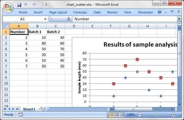
How to Change Excel Chart Data Labels to Custom Values? 05.05.2010 · I Have 4 columns of data to plot. Sounds easy, right? This is the only page in a new spreadsheet, created from new, in Win Pro 2010, excel 2010. Cols C & D are values (hard coded, Number format). Col B is all null except for “1” in each cell next to the labels, as a helper series, iaw a web forum fix.

34 Label Scatter Plot Excel - Labels For Your Ideas
Excel Custom Chart Labels - My Online Training Hub Step 1: Select cells A26:D38 and insert a column Chart. Step 2: Select the Max series and plot it on the Secondary Axis: double click the Max series > Format Data Series > Secondary Axis: Step 3: Insert labels on the Max series: right-click series > Add Data Labels: Step 4: Change the horizontal category axis for the Max series: right-click ...

How to Make a Scatter Plot in Excel to Present Your Data
Apply Custom Data Labels to Charted Points - Peltier Tech With a chart selected, click the Add Labels ribbon button (if a chart is not selected, a dialog pops up with a list of charts on the active worksheet). A dialog pops up so you can choose which series to label, select a worksheet range with the custom data labels, and pick a position for the labels.
Excel::Writer::XLSX::Examples - Excel::Writer::XLSX example programs. - metacpan.org
How to add data labels from different column in an Excel chart? Please do as follows: 1. Right click the data series in the chart, and select Add Data Labels > Add Data Labels from the context menu to add data labels. 2. Right click the data series, and select Format Data Labels from the context menu. 3.

Improve your X Y Scatter Chart with custom data labels
How to create Custom Data Labels in Excel Charts Click on the Plus sign next to the chart and choose the Data Labels option. We do NOT want the data to be shown. To customize it, click on the arrow next to Data Labels and choose More Options … Unselect the Value option and select the Value from Cells option. Choose the third column (without the heading) as the range.
31 Label Scatter Plot Excel - Label Design Ideas 2020
How to Add Labels to Scatterplot Points in Excel - Statology Step 3: Add Labels to Points. Next, click anywhere on the chart until a green plus (+) sign appears in the top right corner. Then click Data Labels, then click More Options…. In the Format Data Labels window that appears on the right of the screen, uncheck the box next to Y Value and check the box next to Value From Cells.
How to Make a Scatter Plot in Excel | Itechguides.com
Excel Charts: Creating Custom Data Labels - YouTube In this video I'll show you how to add data labels to a chart in Excel and then change the range that the data labels are linked to. This video covers both W...
A complete guide to 3D visualization device system in R - R software and data visualization ...
Dynamically Label Excel Chart Series Lines - My Online Training … 26.09.2017 · Great question. Pivot Charts won’t allow you to plot the dummy data for the label values in the chart as it wouldn’t be part of the source data, so the options are: 1. create a regular chart from your PivotTable and add the dummy data columns for the labels outside of the PivotTable. Not ideal if you’re using Slicers.
Post a Comment for "43 custom data labels excel 2010 scatter plot"